Summary

EMSolution has provided various functions for handling magnetic properties, such as "Analysis using nonlinear two-dimensional anisotropic magnetic properties" and "Hysteresis analysis with Play model".
Here, the analysis example using Inverse Jiles-Atherton Vector Hysteresis model, which is a conventional feature of EMSolution, will be explained.

Explanation

In the Jiles-Atherton Model, a well-known hysteresis model, the magnetic flux density $B$ is expressed as a function of the magnetic field strength $H$. To make the $A$-$\phi$ method easier to apply, the model modified to express $H$ as a function of $B$ is the Inverse Jiles-Atherton Hysteresis Model. Furthermore, a vectorized (two-dimensional) model is the Inverse Jiles-Atherton Vector Hysteresis model.
In the Inverse Jiles-Atherton Vector Hysteresis model, given $B$ and H at the current time, $dH$ is obtained for the variation in $dB$. Hence, the hysteresis loop is a local memory with respect to $B$ and $H$, and does not depend on previous history. The data setup is simple, as there are only 5 fitting parameters per direction, but several improvements have been proposed to identify them for real measurement data. For example, the anhysteretic magnetization curve, which is assumed to be a Langevin function, can be changed to a function with better approximation accuracy, or the parameter that is assumed to be a constant can be made a function of magnetic field strength. It has been pointed out in some papers that the Inverse Jiles-Atherton Vector Hysteresis Model implemented in EMSolution cannot correctly represent minor loops because it is a basic model. We believe that this model can be fully utilized depending on the equipment to which it is applied, although it is limited to the analysis of major loops only.

Hysteresis analysis of ring models

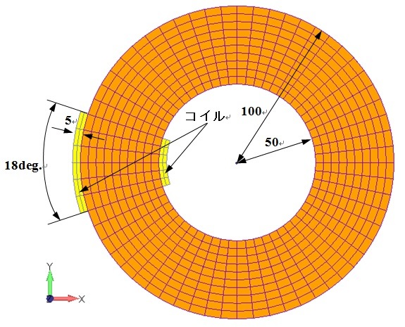
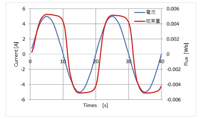
The ring model shown in Figure 1 is used for hysteresis analysis of a two-dimensional static magnetic field. In the ring model, the antimagnetic field is small and the characteristics of the magnetic properties are pronounced. First, a coil current is applied to the demagnetized magnetic ring to determine the magnetic flux density of the magnetic material. The coil current is linearly increased from zero to a maximum value and then decreased to zero.
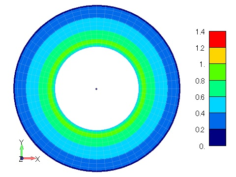
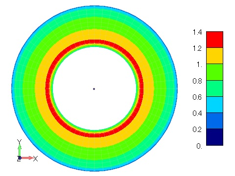
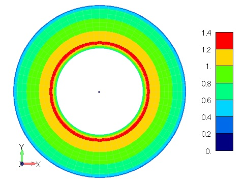
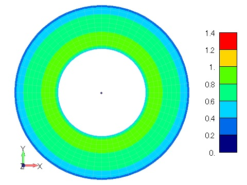
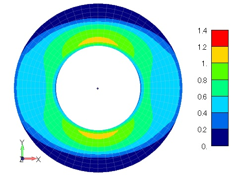
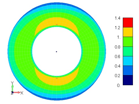
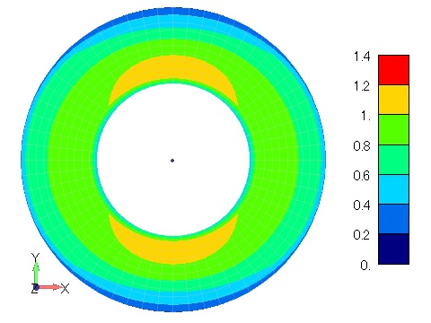
Figure 2 shows the time variation of the magnetic flux density distribution when the magnetic properties are isotropic hysteresis. The magnetic flux density distribution is concentric and constant in the circumferential direction, confirming isotropy. Since this is a hysteresis analysis, the behavior is different when the coil current is rising and falling due to the effect of residual magnetization, and residual flux can be seen even at (d) 10s, when the coil current is zero. The process of this analysis corresponds to the magnetization and demagnetization processes, and if this hysteresis model can be identified with the magnet characteristics, it may be possible to simulate the magnetization and demagnetization processes of a magnet. Figure 3 shows the magnetic flux density distribution for anisotropic hysteresis with the X direction as the rolling direction, and the bias of the magnetic flux density distribution can be seen in the X and Y directions.

Figure 1 Ring model (unit: mm)

(a) 2.5s

(b) 5s

(c) 7.5s

(d) 10s

Figure 2 Magnetic flux density distribution
in a ring model with isotropic hysteresis [ $T$ ]

(a) 2.5s

(b) 5s

(c) 7.5s

(d) 10s

Figure 3 Magnetic flux density distribution
in a ring model with anisotropic hysteresis [ $T$ ]

Figure 4 Hysteresis magnetic properties

Figure 5 Time variation of current and magnetic flux quantity

I briefly introduced hysteresis analysis using the Inverse Jiles-Atherton Vector Hysteresis Model, which is similar to the Play model, the hysteresis model implemented in EMSolution, and can be used to identify the hysteresis model. Since the number of fitting parameters is small, we believe that it can be used for preliminary studies or simple studies of the effects of hysteresis.

How to use

Asymmetric solver settings

For hysteresis analysis using the Jiles-Atherton model, the coefficient matrix is asymmetric, so the asymmetric solver is set up in MATRIX_ASYMMETRICITY (Handbook Section 3.2.6).
Note that applying the line-search method (Handbook Section 3.2.5) to nonlinear analysis is expected to improve the convergence characteristics.

* TREE_GAUGE * REGULARIZATION * RENUMBERING * SCALING * LINE_SERACH * MATRIX_ASYMMETRICITY * -1 0 0 0 1 1

Set up of two-dimensional hysteresis magnetic anisotropy with Jiles-Atherton model

Set ANISOTROPY=4 (Handbook 16.1.1 "Volume Element Properties") to indicate that this is a magnetic material to which the Jiles-Atherton model applies. On the next line, enter the global coordinate system (or local coordinate system) COORDINATE_ID, the specific permeability MU_Z in the Z direction, and the calculation width DB_CAL($T$) of the magnetic flux density. Smaller values of DB_CAL generally result in higher accuracy, but at the cost of more computation time per nonlinear iteration. Enter the magnetic properties in the X and Y directions, starting with the next line. The following values are entered: saturation magnetization (MS), coercive force (K), weight function (C), anhysteretic shape function (A), and coupling coefficient (ALPHA).

* MAT_ID * POTENTIAL * B_H_CURVE_ID * SIGMA * MU * PAKING * ANISOTROPY * 1 0 0 0.0 0 0 4 * COORDINATE_ID * MU_Z * DB_CAL * 0 1.0 0.0001 * MS * K * C * A * ALPHA * ←X方向 1.39E+6 77.51 0.19222 84.96 218.22E-6 * MS * K * C * A * ALPHA * ←Y方向 1.40E+6 72.14 0.13334 144.56 206.66E-6

Download

Ring Materials　　Sample data DL
・ input.ems
・ pre_geom2D.neu