Summary

In the past, EMSolution had a function to output magnetic fluxes chained to an arbitrary closed curve loop, but it was necessary to define the closed curve as a loop connecting nodes entered by nodal numbers or a loop using line elements. However, these could only be defined in a three-dimensional analysis, not in a two-dimensional analysis. We are pleased to report that it is now possible to define arbitrary closed curves with face elements.

Explanation

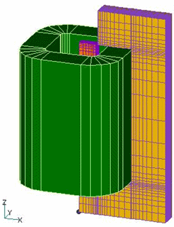
This function is used not only to determine the magnetic flux chained to an arbitrary surface, but also to output the normal component of the magnetic flux density (the flux chained to the surface divided by the area) for each surface element. The plunger model of TEAM Workshop Problem 20 used in the EMSolution benchmark test, shown in Fig. 1, is used to introduce this function.

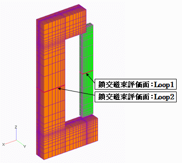
A coil is wound around a magnetic pole, and the coil is defined by COIL. The analysis is a static magnetic field analysis, and currents of 1,000, 3,000, 4,500, and 5,000 A are applied to the coil. The evaluation plane is the pole-center cross-section shown by the red line in Fig. 1(b). The closed curve loop and the surfaces are defined at the same location, and the direction of the closed curve loop is aligned with the direction of the face elements. Note that the closed curve loop must have the same line element direction for each computation loop, and the face elements must have the same face direction for each face element. In the case of node number input, the order of the input node numbers must be the order of the nodes that make up the line elements, i.e., the closed curve. Since this model is a one-quarter model with X=0 and Y=0 symmetry planes ($B_n$=0), there is no need to define line elements on the X=0 and Y=0 planes. The same is true for the node number input, but the result will be the same even if they are defined.

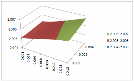
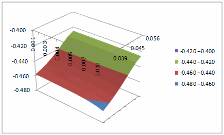
Table 1 shows the results of the fluxes for the node number input, the line element input, and the plane element input, respectively. In this case, the output file contains only the value of the mesh-defined area, so Loop1 is actually 4 times larger and Loop2 is 2 times larger than Loop1. The surface element input also outputs the average magnetic flux density, which is the chaining flux divided by the total area of the face element, so that is also shown. You can see that all results agree. The average flux density shows that Loop1 reaches 2T at an applied current of 4,500A, indicating that it is saturated. As described in "Handling of Inductance in External Current Field Source (COIL)", when compared to the inductor chain flux, it is 4.42233e-004/(1.25318e-004 x 4) = 88.22% at 4,500 A applied, which means that about 88% of the inductor chain flux passes through the iron core and the rest leaks.

Fig. 2 shows the normal component (Bn component) of the magnetic flux density in the face element at an applied current of 4,500 A. The vertical axis represents the magnetic flux density, and $B_n$=$B_z$ from the plane of definition. In Loop 1, the magnetic flux density is almost 2T, slightly biased toward the X=0 plane, and in Loop 2, it is biased toward the Y=0 plane, but as in Loop 1, the values are almost the same.

Table.1 Chain flux results (computational domain)

		Node number input	Line Element input	Surface Element input
		Chain flux (Wb)			Average magnetic flux density (T)
1000A	Loop1	4.42284E-05	4.42284E-05	4.42284E-05	7.07654E-01
	Loop2	-4.16667E-05	-4.16667E-05	-4.16667E-05	-1.33333E-01
3000A	Loop1	1.11718E-04	1.11718E-04	1.11718E-04	1.78749E+00
	Loop2	-1.12385E-04	-1.12385E-04	-1.12385E-04	-3.59632E-01
4500A	Loop1	1.25318E-04	1.25318E-04	1.25318E-04	2.00510E+00
	Loop2	-1.37195E-04	-1.37195E-04	-1.37195E-04	-4.39023E-01
5000A	Loop1	1.28069E-04	1.28069E-04	1.28069E-04	2.04910E+00
	Loop2	-1.43926E-04	-1.43926E-04	-1.43926E-04	-4.60565E-01

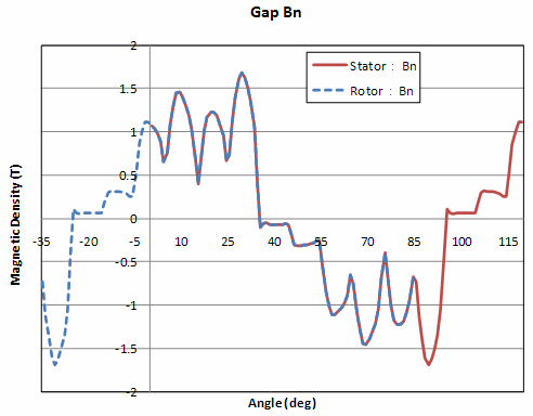
Next, let’s define the chained flux surface using a two-dimensional mesh. We will apply it to the IPM motor model, which was also used in "Fast Convergence to Steady-State Solutions of Time-Periodic Problems" (Fig. 3). For simplicity, we will use a two-dimensional model for the current source analysis and assume the maximum torque operating condition. When performing an analysis using a two-dimensional mesh created in the XY-plane, a three-dimensional analysis is performed inside EMSolution using a three-dimensional mesh that is further extended in the Z-axis direction. Therefore, if a line element is defined on a sliding surface, it will be treated as a plane element with a further extension internally. Using the surface element input for the chain flux shown earlier, the radial component (R component) of the gap flux density, which is the normal component of the flux density of the defined surface, can be calculated. In this calculation, line elements are defined on both the stator and rotor sides for confirmation. Note that if a line element for surface output is defined in the gap, the chain flux and average flux density of the defined surfaces on the stator and rotor sides will be different depending on the angle of the rotor, so it is not considered to be meaningful. Since the gap flux density, which is the normal component of the surface element, is an important parameter in rotating machine design, the purpose is to output this.

Fig. 4 shows the magnetic flux density in the R-direction of the rotor and stator from the static magnetic field analysis results at a rotor angle of -35 degrees (d-axis direction). The rotor side is shifted by -35 degrees and the area of two poles is shown. The stator side and the rotor side are in good agreement. In this way, the same output can be obtained for transient analysis.

From the above, we have shown that, in 3D analysis, as with the conventional input methods of node number input and line element input, input using plane elements can output the normal component of the magnetic flux density of the defining surface in addition to the chain crossing magnetic flux and the average magnetic flux density. Furthermore, we have shown that it is possible to calculate the magnetic flux density in the direction normal to the defining surface even in a two-dimensional analysis. Although these can be calculated using post-processing software from the post data, we hope that you will use this method since it is easier to obtain than using post-processing software.

How to use

As described in "Handbook 11.2 Calculation of magnetic flux linkage”, set MAG_FLUX (11.1) = 1: On and set the following columns for the printed output. NO_LOOPS: Number of defined loops, READ_OPTION: Input method, where READ_OPTION=0: Node number input, =1: Line element input, =2: Face element input.

* MESH * A * V * B * B_INTEG * J_Q * 0 0 0 0 0 0 * Q_AVERAGE * HEAT * MAG_FLUX * CUR_FLUX * 0 0 1 0 * FORCE_J_B * FORCE_NODAL * MAGNETIC_ENERGY * IRON_LOSS * 0 0 0 0 ・・・ * NO_LOOPS * READ_OPTION * 2 0 or 1 or 2

(1) READ_OPTION=0: Node number input

Node numbers are defined in the order in which closed curve loops are drawn.
Note : The nodal numbers for "NODE_IDS" should be on one line.

* NO_LOOPS * READ_OPTION * 2 0 * NO_NODES * 15 * NODE_IDS * 22733 22771 22809 22847 ・・・ 22959 22958 22957 22956 22955 22954 22953 * NO_NODES * 33 * NODE_IDS * 22754 22792 22830 22868 ・・・ 22974 22936 22898 22860 22822 22784 22746

(2) READ_OPTION=1: Line element input

Defines the property number defined for line elements.
Note : Property numbers for "LINE_MAT_ID" should be written on a single line.

* NO_LOOPS * READ_OPTION * 2 1 * LINE_MAT_ID * 51 * LINE_MAT_ID * 52

(3) READ_OPTION=2: Face element input

Defines the property number defined for face elements.
Note : Property numbers for "MAT_IDS" should be on a single line.

* NO_LOOPS * READ_OPTION * 2 2 * MAT_IDS * 61 * MAT_IDS * 62

In the case of a face element input, the average flux density "Average of B on surface (T)" is output in addition to the magnetic flux linkage "Magnetic flux (Wb)" in the output file. In addition, the normal component of the magnetic flux density of the defined face is output in the newly created flux file. Since this data is mesh-dependent, it is output in a fixed format in the "flux" file.

************************************************************************ * Time= 1.00000e+00 * ************************************************************************ No.Loop No X(m) Y(m) Z(m) B_normal(T) 61 41561 1.35734e-03 6.26470e-04 7.50000e-02 7.04245e-01 61 41562 3.84580e-03 6.26470e-04 7.50000e-02 7.05083e-01 61 41563 5.91952e-03 6.26470e-04 7.50000e-02 7.06395e-01

The following information is output at the beginning of the file: Time: time, No.Loop: defined surface property number, No: element number, X, Y, Z(m): surface element center coordinates, B_normal(T): flux density normal component. Even when defined on the rotor side (rotor_mesh(2D)), the element center coordinates are output as the coordinates at the time of mesh creation, so please move them according to the motion distance. This function is performed at the time of POST_PROCESSING and can be used regardless of the calculation contents. If you want to output the data after the calculation, set the nodal number input accordingly, define line and plane elements in the pre_geom(2D) mesh so that the nodal number does not change, and set PRE_PROCESSIONG=1 and MAKING_MATRICES=1 at the time of recalculation. SOLVING_EQUATION=0, POST_PROCESSING=1.

Download

Poblem20

Sample data DL

・ input_nodes.ems : Input node number
・ input_lines.ems : Line element input
・ input_surfaces.ems : Surface element input
・ pre_geom.neu : Mesh data

IPMモータ

Sample data DL

・ input2D_40_5_static.ems : Static magnetic field analysis
・ pre_geom2D.neu : Stator
・ rotor_mesh2D.neu : Rotor