Summary

EMSolution has a function to calculate the magnetic field by spatial integration of magnetization and current based on the Biot-Savart law, which has been evaluated as more accurate than the magnetic flux density obtained by interpolation from elements and nodes. However, it did not support two-dimensional translational analysis (defined in the XY plane with infinite length in the Z direction). Now, it can be applied to 2-D translational analysis as well, which will be explained using an example.　We will also explain how to use it in a two-dimensional axisymmetric analysis.

Explanation

Two-dimensional translational analysis

Two-dimensional magnetic field integration from magnetization and current is performed by the equation below.

$$\mathbf{B}(\mathbf{r}_{p}) = \frac{\mu_{0}}{2\pi} \int_\Omega \left( \frac{ \mathbf{J}(\mathbf{R}) \times \mathbf{r}}{r^2} – \nabla_{0} \left( \frac {\mathbf{M}(\mathbf{R}) \cdot \mathbf{r}} {r^2} \right) \right)dS$$　　

$$\mathbf{r} = \mathbf{r}_{p} – \mathbf{R} , r = |r| $$　　

As in the three-dimensional case, $r_p$ is the coordinate of the spatial point for which the magnetic field is to be obtained and $R$ is the coordinate of the integration point. In a two-dimensional analysis, only the $J_z$ component needs to be considered, so the integral term for the current can be simplified. A simple model (Fig. 1) provides an example. The model consists of a linear magnetic material (specific permeability 1000) and a coil, with spatial points of evaluation on top of the magnetic material. A static magnetic field analysis is performed and Fig. 2 shows the magnetic flux density output as a nodal quantity at the space point coordinates and the magnetic flux density obtained from the field integrals of magnetization and current for each component. It can be seen that they are in good agreement, although there are some differences. In particular, there is a large difference in the By component, but this is due to the rather coarse mesh of the coil and magnetic material and, as mentioned in “Magnetic field by integration of magnetization and current”, the far boundary of the FEM mesh, since this is an open domain problem. As the far boundary mesh is elongated, the magnetic field calculated from the magnetization and current does not change, but the results obtained from the FEM asymptotically approach the results from the magnetization and current integrals.

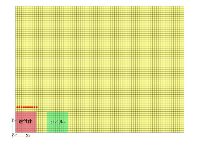
Fig.1 Two-dimensional model
(Red circles indicate integration points)

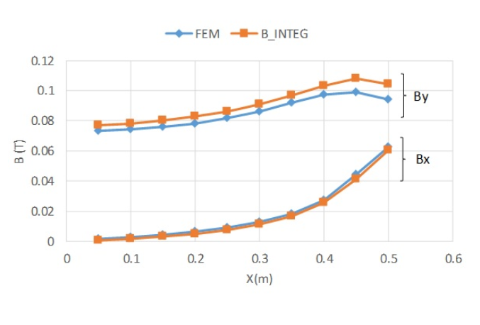
Fig.2 Magnetic flux density on y=0.6m line

Two-dimensional axisymmetric analysis

The model in Fig. 1 is redefined in the ZX plane to perform a two-dimensional axisymmetric analysis. The integrals of magnetization and current in cylindrical coordinate systems are complicated by the use of full elliptic integrals [Ref.1]. Therefore, we will use rotational periodic symmetry and the rotational periodic symmetry in the integrals of magnetization in our calculations.
In EMSolution, one layer of mesh is created in the angular direction for two-dimensional axisymmetric analysis, and the analysis is performed as a three-dimensional mesh. If we extend the mesh in the angular direction by 1 degree, the periodic symmetry of rotation becomes 360. With this set up, the magnetic field integrals for magnetization and current are calculated. Fig. 3 shows the magnetic flux density output as a nodal quantity in spatial point coordinates as in Fig. 2, and the magnetic flux density obtained from the field integrals of magnetization and current for each component. It can be seen that they are in good agreement, although there are some differences in this case as well.

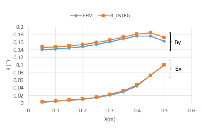
Fig.3 Magnetic flux density on z=0.6m line

References

[1] “Fast Large-Scale Numerical Techniques for Electromagnetic Field Analysis,” Technical Report of the Institute of Electrical Engineers of Japan, No. 1043 (2006)

How to use

For two-dimensional analysis, no specific settings are required. Enter the symmetry data for B_INTEG that matches the FEM boundary conditions. For two-dimensional axisymmetric analysis, enter the number of symmetries in the ROTATION of symmetry data B_INTEG in addition to those that match the FEM boundary conditions. Note that it is not necessary to set the periodic boundary conditions of FEM.

For two-dimensional axisymmetric analysis

* XSYMMETRY * YSYMMETRY * ZSYMMETRY * ROTATION * 0 0 -1 360

Download

Two-dimensional analysis

・ input.ems : Input condition file
・ pre_geom2D.neu : Mesh file

Two-dimensional axisymmetric analysis

・ input.ems : Input condition file
・ pre_geom2D.neu : Mesh file