Summary

There are various types and applications of electrical equipment, some of which use Curie temperatures, in which magnetic materials lose their magnetism above a certain temperature. When analyzing electromagnetic fields of such devices, temperature-dependent analysis of magnetization characteristics (BH curve) is considered effective. This section describes the analysis function to consider temperature dependence of BH curve.

Explanation

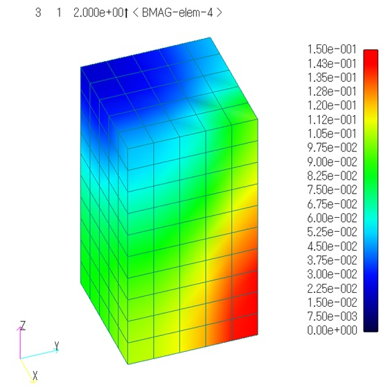
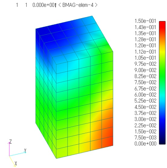
Since there is no suitable temperature-dependent magnetization property, we use the model used in "Non-linear staticmagnetic field analysis" to show an example of a temperature analysis of a magnetic material. The temperature-dependent BH curve used is appropriately set so that the magnetization property worsens with temperature. Figure 1 shows the magnetic flux density distribution at room temperature and at high temperature. At high temperature the temperature of the elements is set so that the outer side (upper side in the figure) is hotter than the center (lower side in the figure). You can see that the distribution is different because the temperature-dependent BH curve is used.

(a) Room temperature Constant temperature

(b) High temperature
The outer side (upper side in the figure) is hotter than the center (lower side in the figure).

Figure 1 Magnetic flux density distribution (T)

We introduced this function by using simple model because there is no suitable example for temperature-dependence analysis of magnetization properties. The purpose of this function is to set temperature-dependent BH curve, but it may be possible to analyze the BH curve depending on an appropriate physical quantity other than temperature. We hope you will make use of this function.

How to use

The TEMP_DEPEND module is required to use the temperature-dependent demagnetization analysis function for magnetization characteristics.

* STATIC * STEP * AC * TRANSIENT * MOTION * NON_LINEAR * TEMP_DEPEND * STEADY_CURRENT * 1 0 0 0 0 1 1 0

To use temperature-dependent magnetization characteristics, the element characteristics ANISOTROPY=2 must be set.

* MAT_ID * POTENTIAL * B_H_CURVE_ID * SIGMA * MU * PACKING * ANISOTROPY * 1 0 0 0 1000 1 2

The temperature-dependent BH curves are to be set in the new NO_T_DEPEND _CURVES.

• BH_CURVE_ID : BH curve ID
• NO_DATA : Number of data points in BH curve table
• NO_CURVES : Number of temperature dependent BH curves, valid when TYPE=0
• TYPE=0 : For "Temperature Dependent Analysis of Magnetic Properties".
  Specify B for each temperature with respect to H.
  TYPE=1 :For "Demagnetization Analysis of Permanent Magnets".
  Set BH curve for each temperature.
• TEMPERATURE : Set the temperature of each BH curve to NO_CURVES times.
• H_AT/M : Magnetization strength ($A/m$)
• B_T : Magnetic flux density at each temperature ($T$)

The following data is required for linear interpolation inside EMSolution

• NO_BM_DATA : Number of reference magnetic flux density ($B_m$)
• HM : Reference magnetic field strength ($A/m$)
• TEMPARATURE : Each $B_m$ temperature
• BM : Reference magnetic flux density ($T$)

* NO_CURVES * NO_T_DEPEND_CURVES * NO_2D_B_H * NO_B_H_MAGNET_CURVES * NO_T_DEPEND_B_H_MAGNET_CURVES * 0 1 0 0 0 * BH_CURVE_ID * NO_DATA * NO_CURVES * TYPE * 1 39 5 0 * TEMPERATURE * 20 100 200 300 400 * H_AT/M * B_T * 0 0 0 0 0 0 27 0.01 0.008 0.0064 0.00512 0.004096 58 0.025 0.02 0.016 0.0128 0.01024 10 0.05 0.04 0.032 0.0256 0.02048 153 0.1 0.08 0.064 0.0512 0.04096 185 0.15 0.12 0.096 0.0768 0.06144 205 0.2 0.16 0.128 0.1024 0.08192 ・・・・・・・・ * NO_BM_DATA * HM * 5 1220 * TEMPERATURE * 20 100 200 300 400 * BM * 1.35 1.08 0.864 0.6912 0.55296

The temperature for each element is specified in temperature.dat. The version number at the beginning of the input file must be "r12.0" or higher.

• NO_STEP : Number of steps to set temperature
• TYPE=0 : Set the temperature for each element
  TYPE=1 : Setting method in "Demagnetization Analysis of Permanent Magnets"
  Set the temperature for each property
• NO_DATA : For TYPE=0, the number of elements to be set, and Number of properties to be set with TYPE=1
• INPUT_TYPE=0 : Fixed
• FORMAT=0 : Set in the format described below
  FORMAT=1 : Set in ATLAS format; valid only if TYPE=0
• REDIRECT=0 : Output the contents of temperature.dat to the check file
  REDIRECT=1 : Do not output to the check file
• IDS : Element number (TYPE=0) or property number (TYPE=1)
• TIME : Time, to be set to include the computed time of the input file
• IDS : Temperature (${}^{\circ }C$)

* NO_STEPS * TYPE * NO_DATA * INPUT_TYPE * FORMAT * REDIRECT * 3 0 250 0 0 0 * IDS * 225 226 227 228 229 230 231 ・・・・・・ * TIME * IDS * -1.0 20 20 20 20 20 20 20 ・・・・・・ 0.0 20 20 20 20 20 20 20 ・・・・・・ 1.0 100 100 100 100 100 100 100 ・・・・・・

When setting the temperature for each element, it is useful to specify the temperature in FORMAT=1: ATLAS format if the number of elements is very large. The ATLAS format is the same as the format of post data files (magnetic, current, etc.).

• STEP : Calculation step number and time
• EVAL : Set element number and temperature as element values

* NO_STEPS * TYPE * NO_DATA * INPUT_TYPE * FORMAT * REDIRECT * 3 0 250 0 1 1 STEP 1 0.000000e+00 EVAL 225 2.000000e+01 226 2.000000e+01 227 2.000000e+01 228 2.000000e+01 229 2.000000e+01 ・・・・・・

Download

・ input.ems
・ pre_geom.neu
・ temperature.dat
・ 2D_to_3D